This guide introduces the Wi-Fi physical (PHY) layer through the 20 MHz orthogonal frequency-division multiplexing (OFDM) PHY used in IEEE 802.11a/g. Start with a single-input single-output (SISO) link: one transmit antenna and one receive antenna. This provides a manageable starting point for understanding how a receiver finds a packet, corrects timing and frequency offsets, and estimates the wireless channel.
The focus is the preamble and receiver processing. Medium access control (MAC), networking, security, and newer features such as multiple-input multiple-output (MIMO) and orthogonal frequency-division multiple access (OFDMA) are topics for later study. See Resources for Wi-Fi for the broader overview.
Prerequisites: basic complex numbers, sampled signals, and MATLAB programming. Familiarity with digital modulation is helpful; review the fast Fourier transform (FFT), inverse FFT (IFFT), and cyclic prefix (CP) in the first stage below.
Learning outcome: generate a non-high-throughput (non-HT) OFDM packet, identify its training fields, and use them to investigate synchronisation and channel estimation. Work through the reading and exercises in order, then try the optional hardware activities. The simulation starting point requires MATLAB and WLAN Toolbox; no radio hardware is needed.
0. OFDM
Reading materials:
- Read Section 4.1, 4.2 of Book MIMO-OFDM Wireless Communications with MATLAB.
- Read Chapter 2 of Book Next Generation Wireless LANs 802.11n and 802.11ac
Key learning points:
- FFT and IFFT
- Time domain and frequency domain signals
- Cyclic prefix and its role in a multipath channel
Exercise: Create a vector of 64 frequency-domain samples, apply an IFFT, and prepend the final 16 time-domain samples as a CP. Remove the CP and apply an FFT. This is a generic OFDM exercise; Wi-Fi subcarrier mapping comes next.
Checkpoint: The recovered frequency-domain samples should match the originals to numerical precision. Explain why the CP repeats the end of the symbol rather than adding zeros.
1. Wi-Fi Physical Layer
1.1 Transmitter
Reading materials:
- Chapter 4 of Book: Next Generation Wireless LANs 802.11n and 802.11ac (Focus on Section 4.1 in the beginning).
- Chapter Orthogonal frequency division multiplexing (OFDM) PHY specification of the IEEE 802.11 standard. Download it from IEEE Xplore
- Non-HT PPDU Structure
Key learning points:
- Preamble design including short training symbols and long training symbols
For the 20 MHz non-HT OFDM physical layer protocol data unit (PPDU), follow these fields in order:
| Field | Duration | What to learn |
|---|---|---|
| L-STF: legacy short training field | 8 microseconds | Packet detection and coarse carrier frequency offset estimation |
| L-LTF: legacy long training field | 8 microseconds | Fine timing, fine frequency offset estimation, and channel estimation |
| L-SIG: legacy signal field | 4 microseconds | Signalling the data rate and payload length |
| Data | Depends on rate and payload length | Carrying the encoded payload |
Field definitions and timings: MathWorks Non-HT PPDU Structure.
Exercise: Generate the packet in Section 2 and plot the real part of its L-STF and L-LTF separately. Use the field indices rather than guessing where each field begins.
Checkpoint: Identify the repeated short training sequence and the two repeated long training symbols. Distinguish the L-LTF guard interval from the ordinary data-symbol CP.
1.2 Channel
Reading materials:
- Chapters 1-3 of MIMO-OFDM Wireless Communications with MATLAB. Understand what is multipath channel. Focus on small-scale fading in the beginning.
- MATLAB has modeled the fading channels, which can be found MathWorks documentation
- Propagation Channel Models for Wi-Fi/IEEE 802.11
Key learning points:
- Small-scale fading
- Modelling of multipath channel (frequency selectivity vs flat fading)
- Modelling of Doppler spread (fast vs slow fading)
Exercise: First pass the generated packet through an unchanged channel. Next add complex Gaussian noise, and then try a fixed two-path channel using filter([1; zeros(3,1); 0.5], 1, tx). This places the second path four samples after the first. Plot the magnitude of the channel’s FFT and compare it with a single-path channel. Keep Doppler for a later exercise.
Checkpoint: Explain the difference between noise and frequency-selective distortion, and compare the path delay with the CP duration.
1.3 Receiver
Reading materials:
- The paper Performance Assessment of IEEE 802.11p with an Open Source SDR-Based Prototype, which explains receiver algorithm design, including time synchronisation, frequency-offset estimation, and channel estimation.
Key learning points:
- Packet detection: How to use short training symbols for coarse time synchronisation (autocorrelation)
- Symbol alignment: How to use long training symbols for fine time synchronisation (cross-correlation)
- Carrier frequency offset estimation and correction (autocorrelation)
- Channel estimation using long training symbols
Exercise: Add a known leading delay to the packet and plot a sliding autocorrelation metric using the L-STF repetition. Then introduce a known carrier frequency offset by multiplying sample n by exp(1j*2*pi*offsetHz*n/fs), with n starting at zero. Estimate and correct the offset before estimating the channel from the L-LTF. Start without noise and add it after the basic processing works.
Checkpoint: Compare the detected packet start and estimated offset with the values you injected. For channel estimation, initially use the known packet boundary and a fixed multipath channel; compare estimated and true responses on the occupied subcarriers. This separates channel-estimation errors from synchronisation errors.
2. MATLAB Simulation
Generate a 20 MHz non-HT packet
Run this starting example in MATLAB with WLAN Toolbox. It generates and plots one packet; it does not yet implement a receiver. The random payload represents bits supplied to the PHY, rather than a complete MAC-layer exchange.
rng(0);
cfg = wlanNonHTConfig;
cfg.Modulation = 'OFDM';
cfg.ChannelBandwidth = 'CBW20';
cfg.NumTransmitAntennas = 1;
cfg.MCS = 0;                 % BPSK, rate-1/2 coding: 6 Mb/s at 20 MHz
cfg.PSDULength = 100;        % PHY service data unit length in bytes

bits = randi([0 1], 8*cfg.PSDULength, 1);
tx = wlanWaveformGenerator(bits, cfg);
fs = wlanSampleRate(cfg);
ind = wlanFieldIndices(cfg);

stf = tx(ind.LSTF(1):ind.LSTF(2), 1);
ltf = tx(ind.LLTF(1):ind.LLTF(2), 1);

subplot(2,1,1);
plot((0:length(stf)-1)/fs*1e6, real(stf));
xlabel('Time within L-STF (microseconds)');
ylabel('Real amplitude');
title('Short training field');
grid on;

subplot(2,1,2);
plot((0:length(ltf)-1)/fs*1e6, real(ltf));
xlabel('Time within L-LTF (microseconds)');
ylabel('Real amplitude');
title('Long training field');
grid on;
References: wlanNonHTConfig and wlanWaveformGenerator.
Checkpoint: At the default sample rate of 20 MHz, each training field contains 160 samples. The L-STF has ten repetitions of 16 samples; the L-LTF has a 32-sample guard interval followed by two 64-sample training symbols.
Build the receiver in stages
Use the non-HT reception functions as references for the receiver exercises above. Work through packet detection, coarse frequency correction, symbol timing, fine frequency correction, and L-LTF channel estimation. Keep the same non-HT configuration throughout.
Save a plot or numerical comparison at each stage. Begin with a noiseless packet and known timing, then add one impairment at a time. Once the preamble processing works, extend the receiver to equalise and decode the data, checking that the recovered bits match bits in the noiseless case.
Extension: 802.11n and MIMO
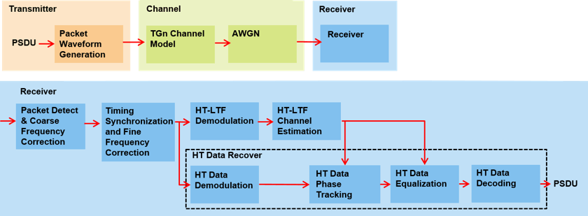
After completing the non-HT exercises, run 802.11n Packet Error Rate Simulation for 2x2 TGn Channel. This uses an HT packet format. Reducing the number of transmit antennas alone does not make it a valid SISO example: the space-time streams, modulation and coding scheme (MCS), and channel transmit/receive antenna counts must also be consistent. Retain the original 2x2 settings initially and compare its processing chain with the non-HT receiver you have studied.
3. Experimental Practice
- Software-defined radio (SDR): if you have SDR platforms (USRP or PlutoSDR), check MATLAB WLAN SDR examples
- ESP32: try ESP32 CSI Toolkit to get CSI
4. WireShark
Using WireShark to monitor the Wi-Fi tranmissions over the air. Check more information at WireShark page
Return to the Main Page of Wireless Communication Technologies.